热力学与统计力学pdf免费版|百度网盘下载

编者评论：热力学和统计力学 pdf

《热力学与统计力学》是世界图书出版公司出版的一本完整实用的现代物理学本科生和研究生教材。它以系统、统一和连贯的方式处理现代理论物理学的各个方面。小编为大家准备了热力学与统计力学pdf版，欢迎下载

读者评论

文笔简洁严谨，让人一眼就能感受到物理学的精髓。这是一本真正的理论物理学高级书籍。热力学中有许多有趣的属性：稀溶液可能过于严格，

其实源于数量和统计效应；比如平均算子，比如齐次函数，这些简单普通的东西在现代数学物理中起着关键作用，这是过去不理解的东西

/p>

什么书热力学

热力学

热力学与普通物理热的最大区别在于，在热力学中，更侧重于热力学量、热机及其效率的引入和测量；而在热力学中，则上升到逻辑推理和推导计算公式的层次。
——沉会川《热物理习题精解》序言

我觉得沉慧川的评论写得很好。就我们上海大学物理系而言，热学包括热物理量的介绍，热力学第1、2、三定律，熵的讨论，气体分子的动力学理论和一阶相过渡。

从气体分子运动学和一阶相变中选择一个，将另一个留给统计物理课程。统计物理分为两个或三个部分，每部分一个半到两个小时，来解释热力学。

不多说，王竹熹绝对是最棒的。很多人可能不知道，王竹熹和P.A.M.狄拉克是兄妹。谁知道。如果他不回国，他可能会获得诺贝尔奖，

或者至少是开创了某个学科的大师（王竹羲有个侄子或者是兄弟，转行成为计算机系的学生，教过一个叫闫乐存的学生）。读本科的时候，这本书看了三四遍。所以一些热力学知识变得直观，往往忽略了学生的痛苦。所以在我的课上，还是要自己多读书，多总结知识图。

统计热力学、统计力学和统计物理学

这三个名字其实是指大二和大三的“统计物理”课程。统计热力学，顾名思义，侧重于统计物理学在热力学中的应用，在理论上并不深究。化学系的名字有很多书。

这个名字可以追溯到薛定谔和理论化学家特雷尔希尔；统计力学，顾名思义，就是用统计方法来研究力学，或者把统计方法应用到力学上，不可能分析出一摩尔气体的作用力，

p>

至少需要一个哈密顿量。统计物理学是一个更广泛的术语，可以在没有哈密顿量的情况下为您提供统计数据。比如张首晟儿子写的Arxiv，就用统计物理学的思路，讨论了岛上土著人拥有椰子的情况。

在吴大友看来，统计物理学包括两个部分：统计方法和动力学理论。我对动力学理论不是很熟悉，所以可以参考《非平衡态统计物理学》和《稀有气体数学理论》等书籍。这里也有一个很好的答案：

关于统计力学的基本原理

宏观系统有几个可直接观察到的量，例如气体压力 p、体积 V 和温度 T。热力学描述了这些量之间的关系，而现象学描述了系统的整体行为。统计力学的目的是研究宏观物体的行为和性质所遵循的一种特殊规律，

它的一项重要任务是将热力学解释为一种现象学理论。统计力学可以从分子的微观性质计算热力学量。统计力学有双重含义：热力学量是从微观力学知识（如分子能级、光谱测量）中计算出来的，

从宏观热力学性质的测量值推断微观性质（例如分子间相互作用）。统计力学可以突破热力学的局限，将研究扩展到热力学不再适用的领域。非平衡系统一般没有简单的热力学宏观描述。

但分布函数的描述仍然是明确的。统计力学处理服从哈密顿动力学的微观系统，但原则上，微观对象也可以是经济量、社会学量等，不满足哈密顿动力学。

1 统计规律

考虑在体积为 V 的空间中有 N 个服从经典哈密顿动力学的粒子，这个系统的状态由这些粒子的坐标和动量决定（r1, r2,···, rN; p1, p2 , ···, pN) ≡ (rN, pN) 给出，这种状态也称为微观构象态或构象态。

构象状态对应于由 rN 和 pN 跨越的 6N 维相空间中的一个点。假设系统哈密顿量为 H(rN, pN) = K(pN) +U(rN)，则运动方程为

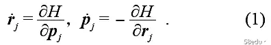
系统的构象状态随时间的演变在相空间中绘制了“相轨道”或分子轨道。这样的系统虽然遵循经典力学，写出运动的微分方程并不难，但其自由度巨大，不可能求解给定的初始条件积分方程。

大量的自由度导致系统出现全新的规律。作为热力学对象的宏观系统总是存在于某种环境中。内在（混沌系统的动态不可预测性）和外在（环境干扰噪声）导致分子轨道之间不断混合。

原来的分子轨道图已经不存在了，也不需要精确求解动力学了。系统中出现了新的规律，即统计规律，例如体积V内任何足够大的体素中的粒子数是相当恒定的。这导致了热力学中的观察：

大型系统表现出非常简单、有序的行为，只需几个变量即可表征。然后分子轨道的语言被分布的语言所取代。统计规律性定义了系统的一种新状态，即统计力学状态，它规定了相空间上的分布，

描述系统在相空间中某一特定点附近出现的概率。需要强调的是，这种统计规律并不依赖于微观规律的具体细节。无论用经典力学还是量子力学来描述粒子的运动，统计力学的理论框架都没有改变。

热力学中热力学平衡的宏观状态是热力学状态，它完全由几个自变量定义，具有相应的热力学状态空间。热力学状态空间中的路径对应于热力学过程。热力学量，其中一些可以通过统计力学分布的平均得到，

其他不是平均数量，必须直接从分布中推导出来，后者需要特别说明。区分构象状态、统计力学状态和热力学状态并不难，有意识地、准确地应用这些概念来思考和分析问题是至关重要的。

2 个规范合奏

系统的统计力学状态是指相空间中的分布。一般来说，分子轨道动态演化的时间尺度远小于分布演化的时间尺度。统计力学系统始终处于环境中，具有很大的自由度，

使得分子轨道动力学的精确解既不可能也没有必要。这也是为什么系统的平衡状态存在简单的宏观热力学描述的原因。一个大自由度的微观系统，作为一个动力系统，除了哈密顿量外，没有其他独立的运动积分。

在理想情况下，系统只有哈密顿量，并且仅在统计平均值的意义上是守恒的。统计力学系统的分布演化的长期行为只能取决于它的哈密顿量。分子轨道的时间尺度和分布的时间尺度相互分离，

这导致时间在平衡统计力学中没有发挥重要作用。上述统计力学原理给出了一个平衡的统计分布作为正则分布。关于规范分布，值得进一步讨论。

Gibbs 在 1902 年引入了集合的概念，集合是满足一定统计分布的物理实体的集合。通过获取整体的统计平均值来计算对象的属性。对于合奏的概念，马耿认为“没有必要，不切实际”。确实，“

Ensemble”充其量只能看作是“distribution”的同义词，将其解释为系统的某种复制集是多余的。实际上，在单个宏观系统的热力学测量的时间尺度上，感知的是统计力学的状态，分布，

物理系统也是通过分发来准备的。由于历史原因，“合”字也没有必要废除，只要与“分布”同义就足够了。 Gibbs 的集成理论是一种公理化表示，它同意如何编写分布函数，无论它来自何处。对于正则分布，可以给出以下对最大熵原理的解释。

假设所有决定系统哈密顿量的外部参数，如粒子数、体积等变量都已给定，则系统在相空间的分布记为P(rN, pN)，并且对系统施加的唯一约束如下 U 是一个固定值：

这里 E 是系统能量。根据最大熵原理，系统的分布应为

这里 Z 被定义为归一化因子或“状态总和”或配分函数，如下所示：

此分布 P(rN, pN) 在唯一约束 U（或当 U 是唯一可测试信息时）下最大化熵

（对于统一的分布，熵等于国家数量的对数，因此可以将熵理解为有效状态数量的对数。玻尔兹曼常数 kB = 1 。分布参数β=1/T，即温度T的倒数或倒数，

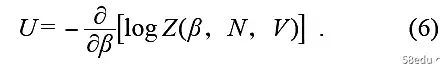
只要不混淆，β也直接称为温度（只是kBT的组合总是出现在统计力学的表达中）。这种分布在统计力学中称为典型集合分布或麦克斯韦-玻尔兹曼分布。平均能量U是热力学中的内能，可以用配分函数Z表示：

统计力学在其环境中研究系统。环境可以是状态预设的测量仪器、其他系统或热水浴。环境的理想模型称为热储层。可以想象它有多少自由度，它具体的粒子组成和动力学并不重要。

本质是它处于一种平衡状态，为其中的系统提供能量交换，而热库的状态在与系统交换能量的过程中不会发生变化，或者说它的状态变化总是微不足道。因此，热储层始终处于平衡状态，其最重要的性质是其温度β。简而言之，热储库是一个恒温的能量池。

值得注意的是，在教科书给出的配分函数定义（4）中，并没有指定积分范围。应该是分布函数(3)的支持。支撑的分配是统计力学计算的第一步，取决于所研究的物理系统和问题。支撑在统计力学中的作用没有得到应有的重视，稍后将进一步讨论。

可验证信息定义了能量均值，即内能，但正则分布的能量有波动。内能可以用配分函数Z对温度β的导数表示，能量的涨落也可以用配分函数Z表示，能量的方差为

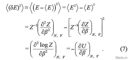
注意等压热容CV =(∂U/∂T)N,V的定义有
<δe>
2 = β-2CV。能量波动与温度的平方成正比，表明它可以作为温度的量度，反映分子轨道的混合程度。

这一结果将能量的自发涨落与温度变化引起的能量变化的响应率联系起来，同时也预示了线性响应理论和涨落耗散定理。

3 个微正则系综

canonical 系综直接描述了 T-V-N 定恒温、定容、定质量系统。具有固定T-P-N和其他集合分布的Gibbs集合分布可以从正则分布推导出来，并且可以证明不同集合之间的等价性。

整体等价的推导要求系统和热浴都很大。正则分布中的体积是固定的，而 Gibbs 系综分布中的体积是波动的，但根据中心极限定理，当系统较大时波动趋于零。

微正则系综，也称为NVE系综，考虑系统能量在以E为中心的无限窄区域内的极限。特别是在原则上，微正则系综看似最简单，但与实际系统并不对应，除了计算上的不便，

熵和温度的定义仍然不明确。在微正则系综中，能量小于E的相体积函数v(E)可以定义三种熵。

相体积函数的定义对于量子力学和经典力学是不同的。通常需要引入一个以E为中心、宽度为ω的归一化核函数，即平滑函数f((H-E)/ω)。在量子力学中，分布由密度矩阵ρ̂表示：

这里Hi和|ψi>是哈密顿量的特征值和特征向量。如果取微正则系综的极限ω → 0，则原始的δ(​​H-E)将是有问题的，因为当能面宽度小于能级区间时，能级计数可能为零。

复杂系统的能级简并几乎只是偶然发生，最终的能级计数随能量值离散变化，导数只能取零或无穷大。因此，需要通过平滑函数 f 来保持能量面的宽度，NVE 系综成为 NVE-ω 系综。

这里C是重复计数校正因子（例如粒子当量），W对应于加宽能量面的有效体积，因此W = ω(dv/dE)。

关于系综和热力学的对应关系，玻尔兹曼只考察了理想气体，吉布斯完成了详细的深入分析。三种熵分别定义为玻尔兹曼熵SB、体积熵Sv和面积熵Ss：

对应的温度可以定义为 1/Tv = dSv /dE 和 1/Ts =1/TB = dSs /dE = dSB/dE。可以从体积熵推导出来

对应于热力学第一定律，虽然从面积熵中可以得到类似的公式，但压力是复杂的，并不对应对应量的平均值。虽然微正则系综的Tv或Ts与ω无关，但仍不能充分发挥热力学温度的作用，

例如，没有指明热流的方向。 （系统1、2及其复合系统的能量分别记为E1、E2和E12=E1+E2、一般来说，dSv1/dE1=dSv2/dE2并不保证dSv1/dE1=dSv2/dE2=dSv， 12 /dE12 .

仅在复合系统微正则系综的平均意义上，dSv,12 /dE12 =

E12=

E12、 ) 它们在处理复合系统方面存在严重困难，并且还具有负温度，因为系统状态密度不一定是单调的。

微正则系综是否等同于其他系综，例如正则系综？从正则系综看微正则系综，当且仅当微正则系综的 E 满足系统的内能 E = U 时，波动被忽略，两个系综等价。阶段

相关文献强调微规范集成通常不等同于其他集成。从规范集成推导出微规范集成很容易找到问题。热力学系统的能量围绕内部能量波动。哈密​​顿动力学的分子动力学模拟，

是能量守恒。这时，系统的总能量应该接近内能才有意义。但是，系统的内能一般是事先不知道且不可控的，因此通常通过缩放平均动能来调节，或者通过模拟恒温器热储库（例如 Nosé-Hoover）的算法来调节。 NH) 恒温器。

4 相变和遍历中断

Ising 模型具有最低能量状态，其中所有自旋在温度 T = 0 时平行排列。由于铁磁相互作用参数 J > 0，相邻自旋方向的排列对能量有益，但这种排序是有害的为熵。然而，在非常低的温度下，

熵对自由能的贡献受到抑制，自旋取向在宏观距离上可能趋于一致，即存在长程自旋相关或长程有序。因此，即使在没有外场的情况下，M≡
<σi σi>
零。这种现象就是自发磁化。可以发生自发磁化的最高温度是伊辛模型的临界温度。

没有磁场的伊辛模型关于自旋的上下方向是对称的。似乎 M 的精确计算只会导致零，因为对于总自旋 m = Σi σi 为正的每个配置，必须有另一个 m 为负的对称配置，相互抵消。

自发磁化的对称性破缺是如何发生的？一种机制是引入一个“辅助场”，从中获得对称破缺的初始分布，之后即使辅助场趋于零，对称破缺也可以保持。然而，更自然的机制是遍历中断，如下所述。

定义总自旋m=Σi σi为给定值μ的所有构型之和，“准构型和”y(μ)和“准自由能”g(μ)定义如下：< /p>p>

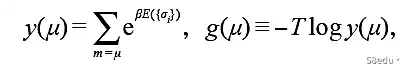
那么配分函数显然是 Y(T,h,N) =Σμ y(μ) =Σμe-βg(μ)，而 y(μ)/Y 是观察到总自旋为微米。从上面关于自发磁化的讨论中，可以假设函数 g(μ) 作为一维有效势能表现如下：

高温时为单阱，温度低于临界温度时为双阱电位。外场会使电位显得不对称，特别是双阱电位的两个阱的深度不相等。重要的是，一旦势垒出现，其高度应根据磁畴表面积估计为~N(d-1)/d，

只要按N的正幂进行缩放，在热力学极限下就会趋于无穷大。除了热力学极限之外，平衡状态还涉及时间趋于无穷大的动力学极限。无限高的障碍会使以下两个限价单不相等：

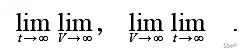
在后一个序列中，只要温度不是极低，系统仍然有机会进入屏障的两侧，而在前一个序列中则没有。对于实际的系统来说，时间和量是有限的，取什么顺序要根据系统的具体流程来决定。简而言之，相变伴随着遍历中断。

在气相或液相的数值模拟中，初始状态一般取一定的均质状态。如果系统的参数对应于气液相变区，类似于伊辛模型的情况，一般不会得到相共存。如果你想得到相位共存，比如在模拟界面行为的时候，

您必须选择非常不同的初始条件，例如让所有粒子都在容器的一侧，然后让系统放松。气相和液相之间最显着的区别是密度，特别是远离临界点。选择合适的截断半径，

将粒子分为气相或液相的标准可以被视为以粒子位置为中心的截断球体中的粒子数。各态的遍历断裂表明，上述两种相对极端的初始构型具有截然不同的演化特征，被标记为气相的粒子会长时间停留在气相中，

液相粒子也是如此。当模拟系统的规模较小时，各状态的遍历断裂现象不是很显着，气体或液体粒子的寿命也不长，而且经常相互切换。随着系统尺寸的增加，气体或液体颗粒的寿命将显着增加。突变是否以及如何发生，值得深入观察和探索。

5 热力学极限和分布支持

最终证明了统计力学与热力学的对应依赖于热力学极限的存在，而这个极限的存在是后验的，与系统哈氏合金量的性质密切相关（Bogolyubov ( 1946)、van Hove (1949)、Yang-Lee (1952)、Fisher-Ruelle (1966))。

以巨正则系综为例，有必要证明极限 limV → ∞V-1 log Ξ 的存在。李阳考虑了一个比较一般的系统哈密顿量，证明了它的热力学极限的存在。耿马提到了李阳证明的可能扩展，并指出李阳二体势不符合电磁相互作用等最重要的物理力。

与标准统计力学教科书一样，在第2节的配分函数定义方程（4）中，没有明确写出积分区域，即没有指定分布函数的支持集。当上一节讨论的遍历突破发生时，物理系统所访问的相空间区域发生了变化，

表示分布函数的支持有相应的变化。如何选择分布函数的支持取决于所讨论的物理问题。例如，如果讨论晶体，必须首先考虑晶格对称性，它定义了分布函数的支持集。

Gibbs 引入了一个巨大的规范系综来处理化学反应系统。以H+H→H2的反应，即氢原子结合成氢分子为例，对比量子力学和统计力学。量子力学从二氢原子的哈密顿量出发，在 Born-Oppenheimer 近似下分离原子核的自由度，

然后求解电子的薛定谔方程，求出电子能级 Ui(R) 作为与原子核距离 R 的函数，然后将束缚态解释为氢分子。在统计力学处理中，氢原子和氢分子必须在一开始就包含在大正则系综中。从纯氢哈密顿量开始，

不可能从统计力学中获得氢分子。纯氢原子体系的相空间不同于氢原子和氢分子混合体系的相空间，这与各态的突破有关。一级相变可以看作是最简单的化学反应 A→B，必须用相应的宏观正则系综来处理。

无论是分子动力学模拟还是蒙特卡洛模拟，分布函数的支持度不变是一个必要的前提。在使用各种加速方法或增强采样方法时应谨慎行事，这在文献中似乎没有得到充分强调。

6 热力学对应：热和自由能

热力学是物理学的一个分支，研究热和温度以及它们与能量和功的关系。它定义了内能、熵和压力等宏观变量，并描述了这些变量之间的一般关系，不涉及特定物质的特定性质。这样的一般规律集中在热力学第四定律中，即第零到第3、

热力学研究的最初动力是提高热机的效率。热力学最基本的概念是系统和环境，最基本的对象是热力学状态和热力学过程。热力学系统是宏观的物理对象。当系统在给定条件下与环境处于热力学平衡时，

状态完全由表示宏观性质的物理化学变量来描述，即状态变量。系统的热力学平衡状态由有限个独立状态变量决定，这些独立状态变量被拉伸到一个热力学状态空间中，其中一个点对应一个状态。状态变量分为强度量和扩展量。

前者随着系统规模或质量的增加或减少而变化，而后者与系统的规模成正比，是可加的。限制状态时，必须至少有一个扩展，否则无法确定系统的大小。熵不符合外延量的直接表示的定义。存在三种类型的热力学量。第一类是外部参数，

属于外部环境，与系统内部状态无关。第二类是系统微观构象动力学函数的平均值。第三类是热力学特有的典型量，可以称为热量。它们没有微观意义，只能在宏观层面把握，属于分布函数。状态方程

，也称为状态方程，描述了热力学系统中不完全独立的多个状态变量之间的关系。热力学过程是与热力学状态空间中的路径相对应的热力学状态的变化。 （非平衡过程没有路径表示。）热力学过程需要仔细定义自变量和因变量。

If the pressure is selected as an independent variable in the isobaric process, it is preset to remain unchanged, and the change in the volume of the dependent variable can be deduced from its change. Thermodynamics is just a phenomenological theory. For example, the equation of state satisfies certain thermodynamic constraints, but cannot be derived from thermodynamics because it is related to the material constitution of the system. Deriving thermodynamic relations and calculating thermodynamic quantities from molecular knowledge is the task of statistical mechanics.

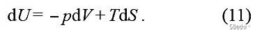
The first law of thermodynamics defines internal energy, dividing it into work and heat, but only internal energy is a state variable, and heat and work depend on the process rather than the state variable. The most common work is the mechanical work Wmech = -pdV, where p is the pressure, the volume decreases when the external work is done on the system, and Wmech is positive. The general form of work is W=Σi fidXi, where fi is the generalized force and Xi is the generalized displacement.

In statistical mechanics, the internal energy U is the average energy:

Here, the probability density is P = e-βE /Z for the regular distribution. At this time, the temperature β and the number of particles N are external parameters, and the volume V is an independent variable. Therefore, the change in internal energy is

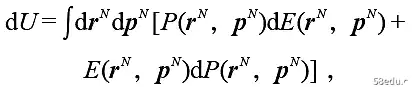
The limitation of the system by the wall of the device leads to the change of the Hamiltonian of the system with volume as dE/dV = -p, where p is independent of the microscopic conformation or configuration, so dE = -pdV, the first term in square brackets gives Work out. By the probability density we have

The second term in square brackets thus corresponds to

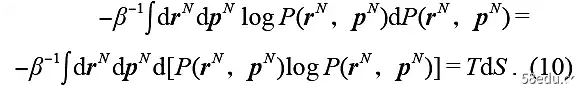
That is, the endothermic term. (It has been considered here that log Z is constant and the probability P is normalized, so the corresponding term of log Z has no contribution.) So far, the first law of thermodynamics has been deduced

This formula can be directly extended to the general form of work. If the number of particles is allowed to change and μ =(∂U/∂N)β,V is introduced, then

Here μ is called the chemical potential, which measures the internal energy added by adding a particle to the system. In summary, the change in internal energy caused by changing the Hamiltonian is work, while the change in internal energy corresponding to a change in distribution is heat.

The second law of thermodynamics, a fundamental assumption that can be applied to any heat-related system, has many different formulations to explain irreversible phenomena in nature. An expression by Clausius is that heat cannot spontaneously travel from cold to hot.

In the language of statistical mechanics, the second law of thermodynamics can be expressed as the minimum principle: the free energy of a system in a thermal reservoir always decreases during the spontaneous process. The "decrease" here indicates the direction of the thermodynamic process, and it means "towards equilibrium", which is beyond the scope of interpretation of equilibrium statistical mechanics. Equilibrium statistical mechanics only expresses the principle of minimum: the free energy of the equilibrium state is the smallest among all states.

To keep the notation simple, the summation is used instead of the integral below. For any two distributions {Pi} and {Qi}, the relative entropy is defined as D(Q, P) = ΣiQilog(Qi /Pi) , using log x ≤ 1 - x , let x = Pi /Qi , it is easy to prove that D( Q, P) ≥ 0,

And the equal sign only holds when {Pi} and {Qi} are equal. Now denote the canonical distribution of the system as {Pi} = Z-1 exp(-βEi) , assuming that {Qi} is another arbitrary distribution of the system. According to the non-negativity of relative entropy, there are

Here

Q is the mean of the random variable X under the distribution Q. Established by the simultaneous equal sign of P and Q, there is

So,

It is the Helmholtz free energy in thermodynamics. Accordingly, the Helmholtz free energy of the general distribution Q can be defined as

According to (13), writable

That is, the free energy of the equilibrium state is the minimum. By the way, the inequality relationship here is consistent with the maximum entropy principle that regular distributions have maximum entropy. It is worth noting that the temperature T that appears in the definition of the free energy FQ is of the equilibrium distribution P, or of the thermal reservoir. That is to say, the free energy of any state is only defined for the system in the thermal reservoir. Using (12) again, we can get

The above formula is the free energy change of the equilibrium process, that is, the reversible process, which can be specially recorded as (dF)rev. Considering the constant temperature and constant capacitance process from non-equilibrium state to equilibrium state, at this time (dF)irrev <(dF)rev = 0 , we can generally write dF ≤ -SdT - pdV + μdN . The definition of the free energy of the general state of the system, that is, the non-equilibrium state, is given above, but the direction of the thermodynamic process tends to be in equilibrium and cannot be derived from the equilibrium distribution.

7 The Arrow of Time: Irreversibility

Macroscopic irreversibility is vividly called the "arrow of time", which dominates all macroscopic phenomena. Microscopic reversibility and macroscopic irreversibility seem to be incompatible, which makes people very tangled. From the perspective of historical development of statistical mechanics, non-equilibrium research represented by molecular kinematics comes first, and equilibrium research comes later. The former involves the details of many microscopic processes such as collisions. Poincaré proved the famous regression theorem: a finite mechanical system will return an infinite number of times to a point that is infinitely close to the initial state. This was the curse that haunted Boltzmann all his life. Gibbs proposed an axiomatic formulation of equilibrium statistical distributions with great success. (Gibbs's work was immediately praised by Poincaré after it was published.) In Gibbs' theory, the spell is missing, but not yet cast out. In fact, microscopic reversibility refers to the evolution of molecular orbitals, while macroscopic irreversibility refers to the evolution of distributions, and the two are not necessarily opposed to each other.

In the summer of 1953, Fermi-Pasta-Ulam (FPU) simulated a one-dimensional nonlinear lattice of coupled oscillators with the then-new computer MANIAC, expecting to see the energy split equally between the different modes, but saw It is the Poincaré reversion phenomenon, which is called the FPU paradox. (Many people now think that the FPU paradox should be called the FPUT paradox, in recognition of the contribution of the Greek-born female scholar Tsingou, who was a programmer at MANIAC at the time.) Fermi's experimental design looks at molecular orbitals, and of course only sees Pang Calais returns. If you want to look at the distribution, you should consider the initial state set and allow for orbital mixing.

Understanding the connection between molecular orbitals and distributions, statistical mechanics is one end and nonlinear dynamics is the other. In terms of how to describe nonlinear dynamics in distribution language, Kolmogorov proposed that a physically meaningful invariant distribution is an invariant distribution that survives after the system adds noise but the noise intensity tends to zero. Baker map: when 0 ≤ x < 1/2, (x', y') = (2x, 1/2 y); when 1/2 ≤ x < 1, (x', y' ) = (2x - 1, 1/2 (y + 1) .) is among the simplest examples of reversible dynamics and is worth demonstrating Kolmogorov's ideas in systems such as kneading maps.

8 Time Evolution of Distribution Function

The statistical mechanical state of the system is a distribution function supported on the microscopic phase space. The distributions processed in statistical mechanics, and the time evolution of macroscopic thermodynamic quantities, take into account time scales that are much larger than the microdynamic time scales of molecular orbitals (in a 6N-dimensional phase space). The Gibbs ensemble theory does not contain time, and stipulates the writing method of the equilibrium distribution function, which only shows that the free energy of the equilibrium state is the smallest compared with the non-equilibrium distribution, but does not indicate that it tends to equilibrium. The Liouville equation, which is essentially equivalent to the molecular orbital dynamics equation, is not a suitable starting point. The principle that the time scales of orbital evolution and distribution evolution are separated from each other in Gibbs theory also applies to general or non-equilibrium distributions. To implement the spirit of the Gibbs equilibrium ensemble theory, it is necessary to give up the attempt to derive the distribution evolution dynamics equation from the molecular orbital dynamics equation, just as it is necessary to re-introduce new principles just like not trying to derive the quantum mechanics Schrödinger equation from the Hamiltonian mechanics equation Characterize the time evolution of a distribution function.

A necessary condition of the distribution evolution equation is that the equilibrium distribution is its stationary solution. The evolution dynamics of the system can be described most naturally and directly by the master equation. The master equation considering the evolution of the distribution is defined by the transition probability T(z → z′):

The transition probability T(z → z′) here is completely determined by the Hamiltonian of the system, which satisfies the following detailed equilibrium conditions:

The above distribution dynamics can ensure that the system tends to a regular equilibrium distribution Peq(z). If it is regarded as the basic principle of statistical mechanics, it can be expressed as follows:

The dynamics of the evolution of the distribution function of a system in a thermal reservoir or environment is described by the master equation (18) satisfying the detailed equilibrium condition (19).

It is worth pointing out that the detailed equilibrium conditions here are for the original 6N-dimensional variables, although the detailed equilibrium conditions may not hold in the reduced variable space.

The transition probability matrix T satisfies ∫dzTk (z′→ z) = 1, and has an eigenright vector 1. If T is irreducible, according to the Perron-Frobenius theorem, its spectral radius is 1, and the eigenleft vector corresponding to the eigenright vector 1 is a positive vector, corresponding to the equilibrium distribution. A generalization of finite Markov chains is the theory of compact transfer operators, including the Krein-Rutman theorem. In addition, discrete time can also be extended to continuous time.

The transition probability T(z → z′) as an operator is usually not Hermitian. It is convenient to introduce the following Hermitianization operator t:

The eigenvectors of the eigenvalue λ of T are denoted as Φλ(z) and Ψλ(z) respectively, let Φ1(z) ≡ Peq(z) , then the eigenvector of t is ϕλ( z) = Φλ(z)/ϕ1(z) , where ϕ1(z) = √Φ1(z) , which corresponds to eigenvalue 1, and all remaining eigenvalues ​​are less than 1.写成Dirac 记号形式，记Ψλ(z) → |Ψλ(z)> ≡ ϕ1(z)|ϕλ(z)> ， Φλ(z) →
<φλ(z)| ≡[ϕ1(z)]-1 <ϕλ(z)| ，则转移算符< p>

此处已约定本征矢归一，正交归一关系可表示作
<ϕμ(z)|ϕν(z)>
=
<φμ(z)|ψν(z)>
= δμν 。任意分布P(z) 对应于

至于约化自由度的描述即物理现象的随机过程描述，与粗粒化程度有关。热力学几乎只适于静态，高频过程更多依赖微观描述。虽然朗之万方程可用于非马尔科夫随机力，但不便处理非线性，而福克尔―普朗克(FP) 方程虽可用于非线性和非平稳情形，但只适于白噪声。借助平衡解Peq ，FP 方程可表作

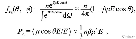
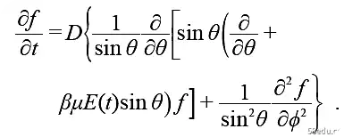
对于在势场U(x) 中的布朗粒子， Peq(x) = Ce-βU ，因而∂tP = ∂x[D(x)(β∂xU+ ∂x)]P 。这样的分布演化方程，满足趋于平衡，漂移项依赖于平衡解，驱动力将含平均场之类的有效场效应。考虑极性分子在非极性溶剂中的稀溶液， 电极化为P =Pd + Pa + Pe ，分别来自偶极取向、距离和电荷分布，后二者在红外和光学高频区有滞后，在慢变场下可吸收入ε∞ ，仅须处理取向项。设密度n 均匀，平衡取向分布为

描述偶极矩的取向布朗运动的福克尔―普朗克方程为

另一例子是核磁共振。响应函数等应可由统计力学导出，并与关联函数联系，表现为涨落―耗散定理。平衡统计力学提供静态响应函数，非平衡统计力学着重讨论动态响应函数的推导。

统计力学必须以某种粗粒化将巨自由度的动力学演化转换为随机演化，其基本问题是给出该转换的数学逻辑，但尚未解决。久保指出，平衡统计力学建立在各态历经上，但进展有限。非平衡远为困难，首先是概念宽泛，须有所限制。两类限制之一是动理学方法，考虑玻尔兹曼型方程，但仅适用于平均自由程足够长，外场频率足够低的情形，不过不限于线性。另一类是近平衡过程，将非平衡性质直接与平衡涨落相联系，不依赖于上述的随机转换，因而可用于随机转换不可行或不必要的情形。后者不假定马尔科夫性或高斯性。二者的适用性有所重叠。 Van Kampen一度曾严批线性响应理论，认为轨道不稳定，微扰计算无据，微观线性与宏观线性完全不同，后者须由玻尔兹曼方程处理。然而，线性响应只微扰处理分布而非轨道，刘维尔方程的确与哈密顿方程等价，但噪声项或扩散项出现后不再等价。轨道不稳定性引起混合导致分布稳定性。动理学理论先随机化而后线性化，线性响应理论则顺序相反。顺便指出，多体微扰项非小量而为O(N) ，宜用约化分布或累积量。

统计力学的核心概念是支在相空间上的分布。统计力学描述的体系，其分布演化的时间尺度远大于相应微观体系的微观态演化或微观轨道的时间尺度。分布演化的动力学方程，不可能由微观态演化方程导出。分布演化方程的一个必要条件是，平衡分布为其长时间演化解。这样的演化方程中驱动项将与平衡分布相关，理论处理的困难不见得来自非平衡，更多地归结于平衡统计力学方法本身的困难。前面曾指出，分布演化方程的一个简单候选，是转移概率满足细致均衡条件的主方程，由之可导出约化的其他形式的方程。